The Energy Game

This is a game that can be played in pairs to explore how the Boltzmann distribution arises naturally from playing with dice and some simple rules. This is played as an introductory exercise of the ‘Molecular Driving Forces’ class imparted by Dr. Ian Gould at Imperial College London.

Consider a planar array of 36 atoms arranged in a 6x6 square. Suppose that each atom may accept one quanta of energy $\epsilon$ . The quanta of energy are moved around randomly using dice throws, and are represented by counters.

Rules of the game

This is a two-person game:

Counters are first placed on the board in any way that the players wish. It is usually convenient to use the 36 counters and to start with one on each square.
The first player throws the two dice. The second player takes a counter off the board from the site given by the coordinates indicated by the two dice. If there is no counter on this square, repeat step 2.
The first player throws the dice again and the second player puts the counter on the square indicated by the dice.
After 5 throws a player draws a distribution diagram, showing the number of squares with 0, 1, 2, 3, … counters on them.
The game continues with distributions diagrams being drawn after 15, 25 and 50 throws.

The objective of the game is to discover the pattern of distribution diagram after many throws. What would we expect the result to be if much larger numbers were used?

An extension of the game is to calculate:

$\Omega = \frac{n!}{\prod_{i=0}^{36}{n_{i}!}}$

After 2, 5, 15, 25 and 50 throws. $n$ is the total number of squares. $n_{0}, n_{1}, n_{2}, ...$ etc. are the number of squares with no counters, one counter, two counters, etc. $\Omega$ is the number of ways of distributing the counters on the board all having the same distribution diagram (also known as multiplicity). It is readily obtained as the number of ways of dividing $n$ objects into groups of $n_{0}, n_{1}, n_{2}, ...$ objects.

Since playing this game can take quite some time, here is an implementation in Python.

import random
import numpy
import matplotlib
import itertools
from matplotlib import pyplot as plt
from scipy.misc import factorial
import seaborn as sns
plt.style.use('fivethirtyeight')
matplotlib.rcParams.update({'axes.labelsize': 12, 'axes.titlesize': 20})

class EnergyGame(object):

    def __init__(self, throws, start):
        self.throws = throws
        self.start = start

    def playGame(self):
        """
        Plays the energy game on a 6x6 grid, with 36 energy quanta

        Parameters
        ----------
        throws: int
            The number of throws to play for
        start: str, 'uniform' (default) or 'skewed'
            If 'uniform', start with one quanta of energy on every atom.
            If 'skewed', place all 36 quanta on the first atom of the array

        Returns
        -------
        number_list, count_list: tuple of lists
            number_list is a list with all the levels that are occupied
            count_list is a list with the corresponding occupance of each level
        """
        # Create table
        if self.start == 'uniform':
            table = numpy.ones(shape=(6, 6), dtype='int')
        elif self.start == 'skewed':
            table = numpy.zeros(shape=(6, 6), dtype='int')
            table[0, 0] = 36
        else:
            raise ValueError('start must be uniform or skewed')
        initial_counters = table.sum()
        succesful_throws = 0
        # Start game
        while succesful_throws < self.throws:
            # First throw
            coords = (random.randint(0, 5), random.randint(0, 5))
            if table[coords[0], coords[1]] > 0:
                succesful_throws += 1
                table[coords[0], coords[1]] -= 1
                # Second throw
                coords2 = (random.randint(0, 5), random.randint(0, 5))
                table[coords2[0], coords2[1]] += 1
        final_counters = table.sum()
        # Do the counting
        number_list = []
        count_list = []
        for number in range(0, int(table.max() + 1)):
            number_list.append(number)
            count_list.append(len(table[table == number]))
        # Conservation of energy checks
        assert sum([st * cnt for st, cnt
                    in zip(number_list, count_list)]) == initial_counters
        assert initial_counters == final_counters
        return number_list, count_list

    def visualize(self, ax=None):
        """
        Visualize the final distribution after playing the game
        """
        if ax is None:
            f, ax = plt.subplots(1, 1, figsize=(7, 7))
        n, c = self.playGame()
        ax.bar(n, c, width=0.5)
        if self.throws < 5000:
            ax.set_title('%d throws' % self.throws)
        else:
            ax.set_title('{:.0E} throws'.format(self.throws))
        plt.setp(ax.get_xticklabels(), visible=True)
        ax.set(xlabel='Count', ylabel='Energy level')
        return ax

Notice that we have added an attribute start to the EnergyGame class, whereby we can explore what happens if we decide to initialize the board in two different ways, either with the quanta of energy spread uniformly across the board, or all stacked up onto one of the squares.

Now that we have the game ready, let’s play!

The game can be played by instantiating an object of the EnergyGame class and calling the visualize method on it:

board = EnergyGame(100, 'uniform')
board.visualize()
plt.show()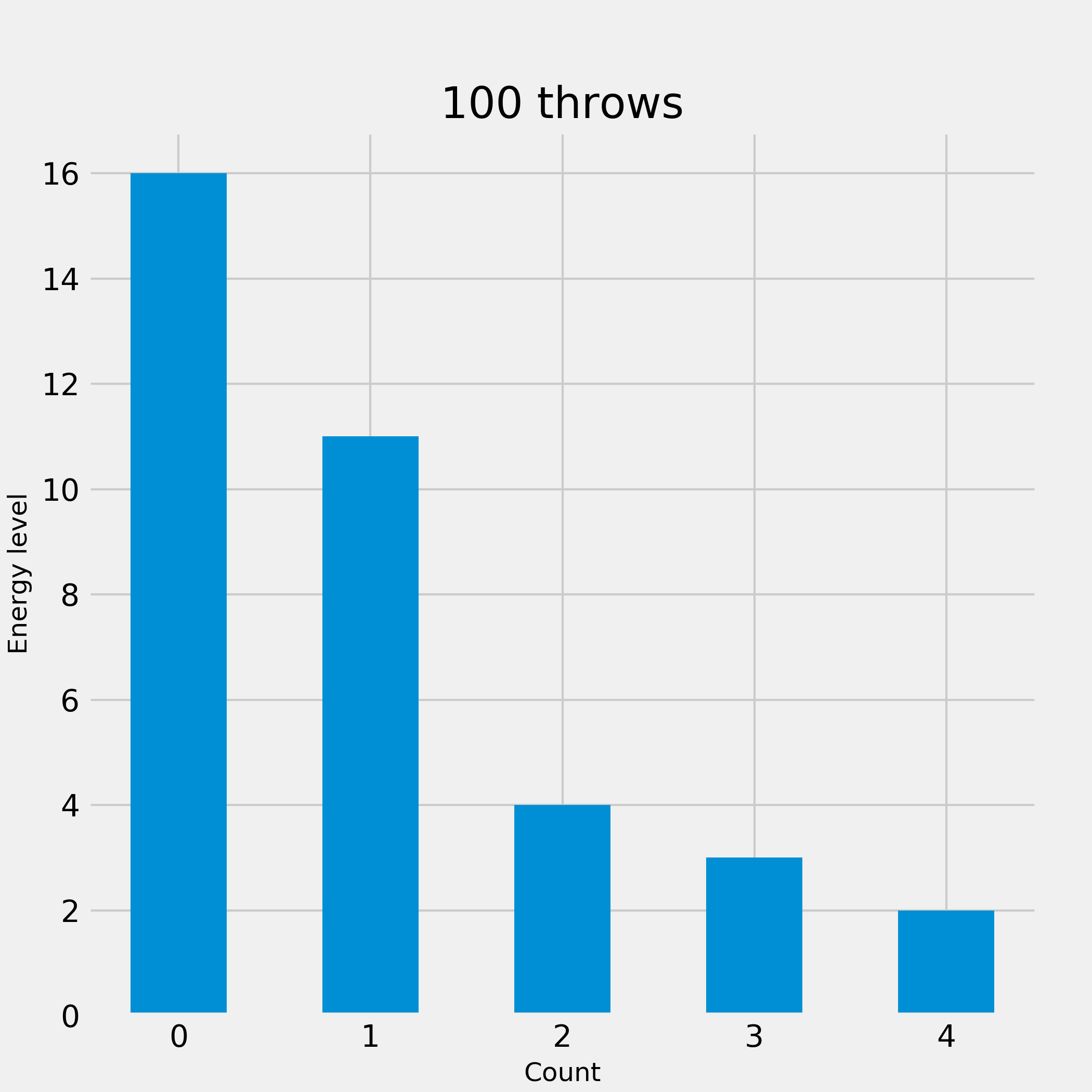

plot0

Let’s use a plotting function that shows how the final distribution changes with the number of throws:

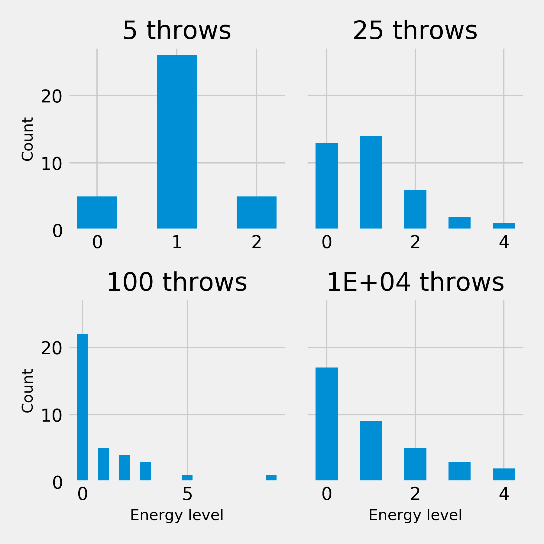
def plot_plays(start):
    f, axarr = plt.subplots(2, 2, figsize=(6, 6), sharey=True, sharex=False)
    for throws, coord in zip([5, 25, 100, int(1e4)], itertools.product([0, 1], [0, 1])):
        board = EnergyGame(throws, start)
        ax = axarr[coord[0], coord[1]]
        board.visualize(ax=ax)
    axarr[0, 0].set_ylabel('Count')
    axarr[1, 0].set_ylabel('Count')
    axarr[1, 0].set_xlabel('Energy level')
    axarr[1, 1].set_xlabel('Energy level')
    plt.tight_layout()
    return f

Here’s what it looks like for a uniform starting board:

plot_plays('uniform').savefig('energy_game_uniform.png', dpi=300)

An exponential distribution is arising, even after only a handful of throws! This is the Boltzmann distribution since the entropy is being maximised under constraints:

$\sum p_{i} = 1$
$\sum E_{i}p_{i} = \langle E \rangle$

plot1

And we see the same behaviour from a skewed initial pose. It just takes longer to achieve because many of our trials are unsuccesful, specially at the beggining, where our dice will keep pointing us towards squares that are empty.

plot_plays('skewed').savefig('energy_game_skewed.png', dpi=300)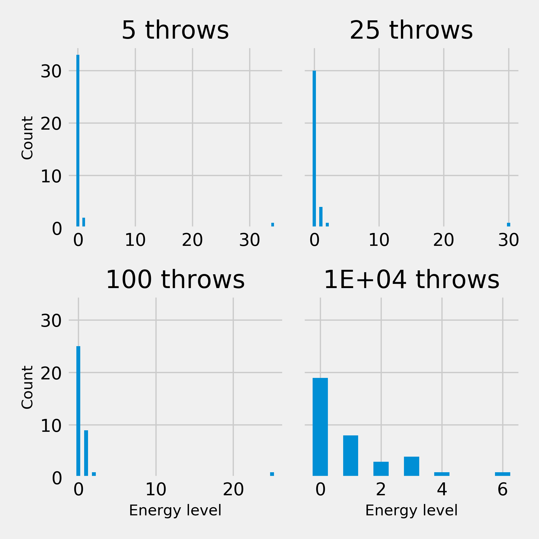

plot2

You can download the game to reproduce the images here