Ideal gas law from a lattice model

I am preparing to be a Teaching Assistant for an undergraduate course of Statistical Mechanics. I am enjoying refreshing my knowledge on this topic by following the Molecular Driving Forces book. In my opinion, it strikes the right balance of theory and applied problems.

One of the examples that has caught my eye at the beginning of the book is Example 6.1, the derivation of The Ideal Gas Law using a lattice model of M sites for N particles and the principle of maximising the Entropy.

After some calculations, one arrives at the following expression:

$P = -kT(\frac{M}{V})\ln(1 - \frac{N}{M})$

Where $\frac{N}{M}$ is the density of molecules. The ideal gas law is now reached assuming that this density is much smaller than 1, by applying the appropiate Taylor expansion:

$\ln(1-x) \approx -x(1+\frac{x}{2}+\frac{x^2}{3} + ... )$

to the first equation, to give:

$P \approx -(\frac{MkT}{V})(-\frac{N}{M})\left [ 1 + \frac{N}{2M} + ...\right ] \approx \frac{NkT}{V}$

I wondered just how small the density has to be for this assumption to hold. Inspired by a recent blog post on how to effectively use the object-oriented matplotlib API, I decided to do some plots of the Taylor expansion to find the region where this is valid.

I first start by doing some relevant imports, setting a plotting style and defining the real and approximation functions that we are going to look at:

from math import log
from matplotlib import pyplot as plt
import numpy
plt.style.use('fivethirtyeight')


def f(x):
    return log(1 - x)


def taylor(x, n):
    total = 0
    for i in range(1, n + 1):
        total += -(1/i)*(x**(i))
    return total

Generate some $x$ values from 0 to 1 and calculate the real value for each one mapping the f function to the numpy.array:

x_r = numpy.arange(0, 1, 0.01)
true_y = list(map(f, x_r))

And we’re finally ready to do some plotting. Notice how the use of map and lambda simplifies a great deal the process of having to generate some data points to plot. No need to use annoying for loops!

# Create two plots on a figure, side by side
fig, (ax0, ax1) = plt.subplots(1, 2, figsize=(10, 5), sharex=True, sharey=False)
# Plot different orders of the Taylor expansion
for n in [1, 2, 5, 10]:
    y_hat = list(map(lambda x: taylor(x, n), x_r))
    ax0.plot(x_r, y_hat, '--', label='taylor_{}'.format(n))
    errors = [abs((true_val - approx_y)*100/true_val) for true_val, approx_y in zip(true_y, y_hat)]
    ax1.plot(x_r, errors, '--', label='taylor_{}'.format(n))

ax0.plot(x_r, true_y, label='$\log(1-x)$', lw=4, ls='-')
ax0.set(xlabel='x', ylabel='y')
ax1.set(xlabel='x', ylabel='error (%)')
ax0.legend()
plt.tight_layout()
plt.show()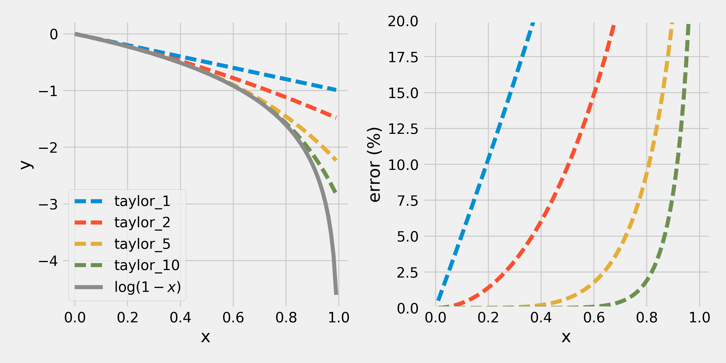

nice_plot

From the right-hand side plot, we can see that the linear function is doing a decent job at approximating $\log(1-x)$ for $x<0.1$ , where the percent error is bound below around 5%. So the Law Of Ideal Gases is acceptable for gases that ocuppy 10% or less of their total available volume.

This is of course nothing new since we’re also assuming that particles of the gases are non-interacting. Modifications to this law like the van der Waals gas law come from keeping the higher-order terms in the expansion.